9 3/27 Lab VIII | Regression Discontinuity Designs

9.1 Preparation
## Packages
library(knitr)
library(haven)
library(tidyverse)
library(rdrobust)

# Load data: data saved as object named "dta"
load("~/GOVT702/Data/Ch11_Lab_AlcoholCrime.RData")
Carpenter and Dobkin (2015) analyzes the relationship between alcohol and crime using a regression discontinuity design.
In this lab we will replicate the results and then explore different specifications. As you will see, some reasonable alternative specifications yield quite different results. The goal here will be to see if we can make any progress in explaining why the results vary as we vary the specification.
From the codebook: “The individual level arrest records are collapsed into arrest counts by age in days for each crime type in the SAS program”P01 Estimate Age Profile of Crime Rates.sas”. This program uses populations estimated from the census in “P00 Estimate Population Denominators.sas” to compute arrest rates per 10,000.”
The main variables are
- all_r: number of arrests across all categories. Our main dependent variable. Arrest data is also broken down for violent_r, property_r, ill_drugs_r and alcohol_r
- post a dumm variable indicating the individual is over 21 years of age
- linear: the number of years from being age 21 (that is, linear = 1.0 indicates 22 year olds. Negative values means the individual is under 21 and positive values indicate the individual is over than 21.
- square: the squared value of linear
- linear_post: interaction of linear and post
- square_post: interaction of square and post
- birthday dummies: e.g., birthday_19 is a dummy for a person’s 19th birthday and birthday_19_1 is a dummy for the day after a person’s 19th birthday. Use this code in your formula: + birthday_19 + birthday_19_1 + birthday_20 + birthday_20_1 + birthday_21 + birthday_21_1 + birthday_22 + birthday_22_1 + birthday_23 + birthday_23_1
See Carpenter, Christopher and Carlos Dobkin. 2015. The Minimum Legal Drinking Age and Crime. The Review of Economics and Statistics. 97:2, 521-524.
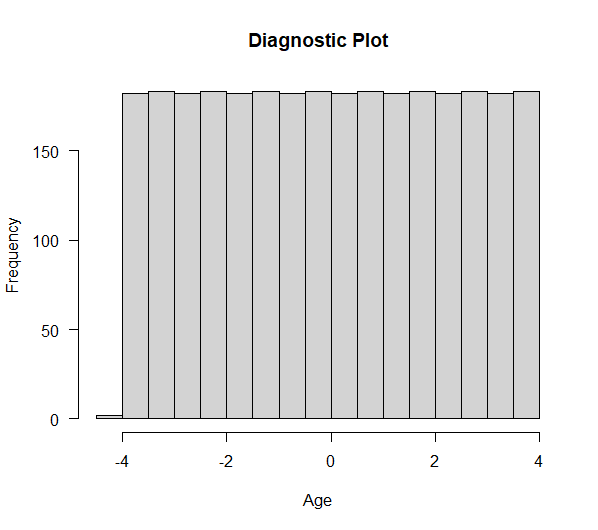
9.2 Run the most basic RDD model and then replicate the main result using the specification for Table 1. In this model, the RD allows for differential quadratic models above and below the threshold and also has dummy variables for birthdays. The data is limited to observations within 2 years of 21. Do this with lm(). Finally, run a diagnostic plot to test for sorting just beyond the cutoff.
## Basic RD model
rd_basic <- lm(all_r ~ post + linear,  data=dta[abs(dta$linear) <= 2, ])
summary(rd_basic)
##
## Call:
## lm(formula = all_r ~ post + linear, data = dta[abs(dta$linear) <=
## 2, ])
##
## Residuals:
## Min 1Q Median 3Q Max
## -89.90 -22.34 -2.25 16.94 695.67
##
## Coefficients:
## Estimate Std. Error t value Pr(>|t|)
## (Intercept) 1534.914 2.537 605.00 <2e-16 ***
## post 76.893 4.536 16.95 <2e-16 ***
## linear -48.792 1.963 -24.86 <2e-16 ***
## ---
## Signif. codes: 0 '***' 0.001 '**' 0.01 '*' 0.05 '.' 0.1 ' ' 1
##
## Residual standard error: 43.34 on 1458 degrees of freedom
## Multiple R-squared: 0.3249, Adjusted R-squared: 0.324
## F-statistic: 350.9 on 2 and 1458 DF, p-value: < 2.2e-16## Differing Slopes
rd_basic <- lm(all_r ~ post*linear, data=dta[abs(dta$linear) <= 2, ])
summary(rd_basic)##
## Call:
## lm(formula = all_r ~ post * linear, data = dta[abs(dta$linear) <=
## 2, ])
##
## Residuals:
## Min 1Q Median 3Q Max
## -89.83 -19.48 -2.83 14.90 671.76
##
## Coefficients:
## Estimate Std. Error t value Pr(>|t|)
## (Intercept) 1559.027 3.043 512.287 <2e-16 ***
## post 76.762 4.298 17.860 <2e-16 ***
## linear -24.712 2.633 -9.386 <2e-16 ***
## post:linear -48.061 3.720 -12.921 <2e-16 ***
## ---
## Signif. codes: 0 '***' 0.001 '**' 0.01 '*' 0.05 '.' 0.1 ' ' 1
##
## Residual standard error: 41.07 on 1457 degrees of freedom
## Multiple R-squared: 0.3943, Adjusted R-squared: 0.3931
## F-statistic: 316.2 on 3 and 1457 DF, p-value: < 2.2e-16## Model with covariates and vary
rd_replicate <- lm(all_r ~ post + linear + square + linear_post + square_post + birthday_19 + birthday_20 + birthday_20_1 + birthday_21 + birthday_21_1 + birthday_22 + birthday_22_1, data=dta[abs(dta$linear) <= 2, ])
summary(rd_replicate)##
## Call:
## lm(formula = all_r ~ post + linear + square + linear_post + square_post +
## birthday_19 + birthday_20 + birthday_20_1 + birthday_21 +
## birthday_21_1 + birthday_22 + birthday_22_1, data = dta[abs(dta$linear) <=
## 2, ])
##
## Residuals:
## Min 1Q Median 3Q Max
## -83.005 -17.601 -0.801 15.893 216.107
##
## Coefficients:
## Estimate Std. Error t value Pr(>|t|)
## (Intercept) 1543.068 2.924 527.744 < 2e-16 ***
## post 91.214 4.146 21.998 < 2e-16 ***
## linear -71.056 6.760 -10.511 < 2e-16 ***
## square -23.726 3.274 -7.248 6.86e-13 ***
## linear_post -16.259 9.573 -1.698 0.0896 .
## square_post 33.666 4.629 7.272 5.77e-13 ***
## birthday_19 287.420 26.396 10.889 < 2e-16 ***
## birthday_20 408.587 26.275 15.551 < 2e-16 ***
## birthday_20_1 217.604 26.275 8.282 2.73e-16 ***
## birthday_21 633.829 26.398 24.010 < 2e-16 ***
## birthday_21_1 673.303 26.396 25.508 < 2e-16 ***
## birthday_22 347.872 26.275 13.240 < 2e-16 ***
## birthday_22_1 382.068 26.275 14.541 < 2e-16 ***
## ---
## Signif. codes: 0 '***' 0.001 '**' 0.01 '*' 0.05 '.' 0.1 ' ' 1
##
## Residual standard error: 26.23 on 1448 degrees of freedom
## Multiple R-squared: 0.7544, Adjusted R-squared: 0.7524
## F-statistic: 370.6 on 12 and 1448 DF, p-value: < 2.2e-16## Diagnostic plot
hist(dta$linear, main = "Diagnostic Plot", xlab = "Age", las=1)
9.3 Run the basic rd model and the model with covariates with library(rdrobust). What is different?
## With RD robust
rd_1 <- rdrobust(x = dta$linear, y = dta$all_r)
summary(rd_1)
## Sharp RD estimates using local polynomial regression.
##
## Number of Obs. 2922
## BW type mserd
## Kernel Triangular
## VCE method NN
##
## Number of Obs. 1461 1461
## Eff. Number of Obs. 164 165
## Order est. (p) 1 1
## Order bias (q) 2 2
## BW est. (h) 0.451 0.451
## BW bias (b) 0.957 0.957
## rho (h/b) 0.471 0.471
## Unique Obs. 1461 1461
##
## =============================================================================
## Method Coef. Std. Err. z P>|z| [ 95% C.I. ]
## =============================================================================
## Conventional 138.387 21.391 6.469 0.000 [96.462 , 180.313]
## Robust - - 6.124 0.000 [98.077 , 190.409]
## =============================================================================summary(rdrobust(x = dta$linear, y = dta$all_r, covs = dta$birthday_19 + dta$birthday_20 + dta$birthday_20_1 + dta$birthday_21 + dta$birthday_21_1 + dta$birthday_22 + dta$birthday_22_1, p=1))## Covariate-adjusted Sharp RD estimates using local polynomial regression.
##
## Number of Obs. 2922
## BW type mserd
## Kernel Triangular
## VCE method NN
##
## Number of Obs. 1461 1461
## Eff. Number of Obs. 160 161
## Order est. (p) 1 1
## Order bias (q) 2 2
## BW est. (h) 0.440 0.440
## BW bias (b) 0.811 0.811
## rho (h/b) 0.542 0.542
## Unique Obs. 1461 1461
##
## =============================================================================
## Method Coef. Std. Err. z P>|z| [ 95% C.I. ]
## =============================================================================
## Conventional 93.650 6.282 14.908 0.000 [81.338 , 105.962]
## Robust - - 13.500 0.000 [81.902 , 109.722]
## =============================================================================9.4 Estimate a series of models with lm() that have slightly different specifications. First, try the above specification with only linear age variable, first fixing slope to be the same above and below the threshhold and then allowing slope to vary above and below the threshhold.
## Additional Models
RD.1 <- lm(all_r ~ post + linear + birthday_19  + birthday_20  + birthday_20_1 + birthday_21  + birthday_21_1 + birthday_22 + birthday_22_1,  data=dta[abs(dta$linear) <= 2, ])
summary(RD.1)
##
## Call:
## lm(formula = all_r ~ post + linear + birthday_19 + birthday_20 +
## birthday_20_1 + birthday_21 + birthday_21_1 + birthday_22 +
## birthday_22_1, data = dta[abs(dta$linear) <= 2, ])
##
## Residuals:
## Min 1Q Median 3Q Max
## -86.028 -20.191 -0.524 18.625 200.851
##
## Coefficients:
## Estimate Std. Error t value Pr(>|t|)
## (Intercept) 1536.997 1.736 885.501 < 2e-16 ***
## post 68.655 3.108 22.089 < 2e-16 ***
## linear -45.492 1.344 -33.836 < 2e-16 ***
## birthday_19 249.713 29.650 8.422 < 2e-16 ***
## birthday_20 416.496 29.620 14.062 < 2e-16 ***
## birthday_20_1 225.573 29.620 7.616 4.7e-14 ***
## birthday_21 662.459 29.650 22.342 < 2e-16 ***
## birthday_21_1 701.818 29.650 23.670 < 2e-16 ***
## birthday_22 344.618 29.620 11.635 < 2e-16 ***
## birthday_22_1 378.755 29.620 12.787 < 2e-16 ***
## ---
## Signif. codes: 0 '***' 0.001 '**' 0.01 '*' 0.05 '.' 0.1 ' ' 1
##
## Residual standard error: 29.6 on 1451 degrees of freedom
## Multiple R-squared: 0.6867, Adjusted R-squared: 0.6848
## F-statistic: 353.4 on 9 and 1451 DF, p-value: < 2.2e-16RD.2 <- lm(all_r ~ post + linear + linear_post + birthday_19 + birthday_20 + birthday_20_1 + birthday_21 + birthday_21_1 + birthday_22 + birthday_22_1, data=dta[abs(dta$linear) <= 2, ])
summary(RD.2)##
## Call:
## lm(formula = all_r ~ post + linear + linear_post + birthday_19 +
## birthday_20 + birthday_20_1 + birthday_21 + birthday_21_1 +
## birthday_22 + birthday_22_1, data = dta[abs(dta$linear) <=
## 2, ])
##
## Residuals:
## Min 1Q Median 3Q Max
## -85.700 -17.549 -0.791 15.896 222.679
##
## Coefficients:
## Estimate Std. Error t value Pr(>|t|)
## (Intercept) 1558.886 1.986 785.091 <2e-16 ***
## post 68.715 2.811 24.445 <2e-16 ***
## linear -23.604 1.720 -13.726 <2e-16 ***
## linear_post -43.777 2.432 -18.002 <2e-16 ***
## birthday_19 271.602 26.842 10.118 <2e-16 ***
## birthday_20 416.496 26.787 15.548 <2e-16 ***
## birthday_20_1 225.513 26.787 8.419 <2e-16 ***
## birthday_21 640.510 26.843 23.862 <2e-16 ***
## birthday_21_1 679.930 26.842 25.330 <2e-16 ***
## birthday_22 344.558 26.787 12.863 <2e-16 ***
## birthday_22_1 378.755 26.787 14.139 <2e-16 ***
## ---
## Signif. codes: 0 '***' 0.001 '**' 0.01 '*' 0.05 '.' 0.1 ' ' 1
##
## Residual standard error: 26.77 on 1450 degrees of freedom
## Multiple R-squared: 0.7439, Adjusted R-squared: 0.7422
## F-statistic: 421.2 on 10 and 1450 DF, p-value: < 2.2e-169.5 Now see what happens when you use a different window sizes. Feel free to experiment (but only need to report one specification.) Just include the treatment and running variables and allow the slopes to differ.
## Different window sizes
RD.3 <- lm(all_r ~ post + linear + linear_post,  data=dta[abs(dta$linear) <= 1, ])
summary(RD.3)
##
## Call:
## lm(formula = all_r ~ post + linear + linear_post, data = dta[abs(dta$linear) <=
## 1, ])
##
## Residuals:
## Min 1Q Median 3Q Max
## -85.20 -21.41 -3.22 15.40 665.30
##
## Coefficients:
## Estimate Std. Error t value Pr(>|t|)
## (Intercept) 1543.846 4.973 310.460 < 2e-16 ***
## post 98.439 7.013 14.036 < 2e-16 ***
## linear -53.881 8.595 -6.269 6.24e-10 ***
## linear_post -33.659 12.131 -2.775 0.00567 **
## ---
## Signif. codes: 0 '***' 0.001 '**' 0.01 '*' 0.05 '.' 0.1 ' ' 1
##
## Residual standard error: 47.4 on 727 degrees of freedom
## Multiple R-squared: 0.2209, Adjusted R-squared: 0.2176
## F-statistic: 68.69 on 3 and 727 DF, p-value: < 2.2e-16RD.4 <- lm(all_r ~ post + linear + linear_post, data=dta[abs(dta$linear) <= 3, ])
summary(RD.4)##
## Call:
## lm(formula = all_r ~ post + linear + linear_post, data = dta[abs(dta$linear) <=
## 3, ])
##
## Residuals:
## Min 1Q Median 3Q Max
## -256.54 -26.50 1.32 30.71 671.72
##
## Coefficients:
## Estimate Std. Error t value Pr(>|t|)
## (Intercept) 1629.580 3.635 448.252 <2e-16 ***
## post 6.250 5.137 1.217 0.224
## linear 54.926 2.097 26.187 <2e-16 ***
## linear_post -127.401 2.964 -42.979 <2e-16 ***
## ---
## Signif. codes: 0 '***' 0.001 '**' 0.01 '*' 0.05 '.' 0.1 ' ' 1
##
## Residual standard error: 60.11 on 2187 degrees of freedom
## Multiple R-squared: 0.4705, Adjusted R-squared: 0.4698
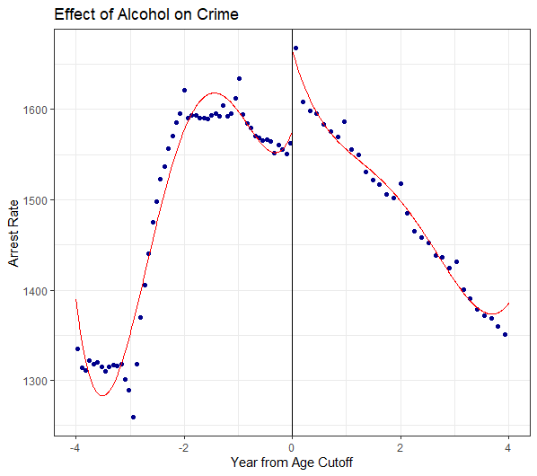
## F-statistic: 647.9 on 3 and 2187 DF, p-value: < 2.2e-169.6 Now create some RDD figures. I suggest using rdplot() in library(rdrobust) and experimenting with different arguments.
## With rdrobust
rdplot(dta$all_r , dta$linear, c=0, kernel = "triangular", x.label = "Year from Age Cutoff", y.label
= "Arrest Rate", title = "Effect of Alcohol on Crime", binselect = "es")
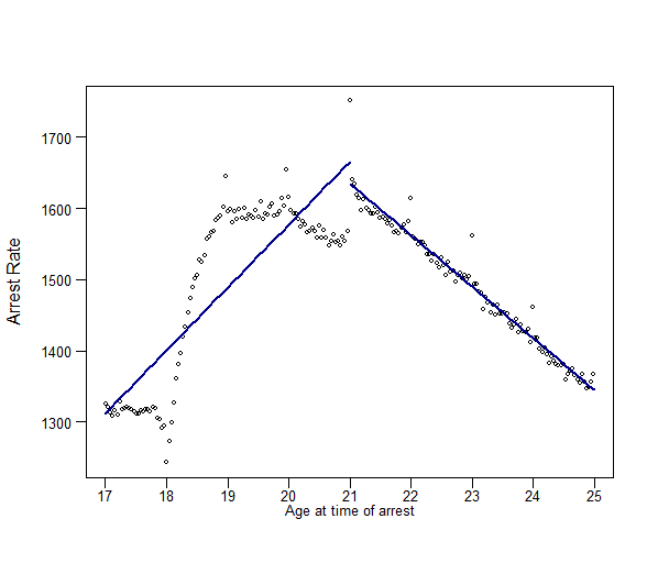
# Create a dataframe that contains average crime rates grouped by bin, limited to the
# window set by the window parameter
dta$age_fortnight = 21 + (14*floor(dta$days_to_21/14))/365

# Create a variable placing each observation in a "bin"
dta$bin  = rep(1:length(unique(dta$age_fortnight)), table(dta$age_fortnight))

window <- 4

dta_bin <-  dta %>%
  select(days_to_21, all_r, property_r, age_fortnight, alcohol_r, bin) %>%
  group_by(bin) %>%
  summarise(property_r_bin = mean(property_r),
            all_r_bin = mean(all_r),
            alcohol_r_bin = mean(alcohol_r),
            age_fortnight_bin = mean(age_fortnight)) %>%
  filter(age_fortnight_bin >= 21- window & age_fortnight_bin <= 21 + window)

# Linear model with varying slopes below and above threshhold
# ALCOHOL ARREST RATES
rd_linear_left <- lm(all_r ~ linear, dta[dta$linear > -window & dta$linear <0, ])

rd_linear_right <- lm(all_r ~ linear, dta[dta$linear  < window & dta$linear >0, ])

# Create a scatter plot
plot(dta_bin$age_fortnight_bin, dta_bin$all_r_bin,  type = "p", pch = 1, cex = 0.5,
     cex.main = 0.8, xlab = "", ylab = "", xaxt='n', yaxt='n')
axis(2, las = 1, tick = T, cex.axis = .8, mgp = c(2,.7,0))
axis(1, tick = T, at= seq(17, 25, by=1), labels =seq(17, 25, by=1),cex.axis = .8, mgp = c(2,.3,0))
mtext("Arrest rate",    las = 1, side = 2, at = 520, line = -0.2, cex = 1)
mtext("Age at time of arrest",  side = 1, line = 1., cex = 0.8)

# Add fitted lines from "left" and "right" models
points(seq(21 - window, 21, by = 0.1), coef(rd_linear_left) [1] +
         coef(rd_linear_left) [2]*seq(-window, 0, by = 0.1), lwd = 2,
       col = "darkblue", type = 'l')
points(seq(21, 21 + window, by = 0.1), coef(rd_linear_right)[1] +
         coef(rd_linear_right)[2]*seq(0, window , by = 0.1), lwd = 2,
       col = "darkblue", type = 'l')