8 Lab VII: Interactions & Categorical Variables

8.1 Categorical Variables and Reference Categories
8.1.2 The Four Categories of the Treatment Variable
unique(social$messages)## [1] "Civic Duty" "Hawthorne" "Control" "Neighbors"8.1.4 Difference in Means Between Categories
reg1$coefficients[1]## (Intercept)
## 0.3145377reg1$coefficients[2]## messagesControl
## -0.01789934reg1$coefficients[3]## messagesHawthorne
## 0.007836968reg1$coefficients[4]## messagesNeighbors
## 0.063410578.1.5 Changing the Reference Category
social$messages <- as.factor(social$messages)

reg2 <- lm(primary2006~relevel(messages, "Control"),
           data=social)

reg2$coefficients[1]
## (Intercept)
## 0.2966383reg2$coefficients[2]## relevel(messages, "Control")Civic Duty
## 0.01789934reg2$coefficients[3]## relevel(messages, "Control")Hawthorne
## 0.02573631reg2$coefficients[4]## relevel(messages, "Control")Neighbors
## 0.081309918.2 Interactions
- How to use interactions
- In R
lm(y~x*z, data=data)orlm(y~x + z + x:z, data=data)
- In R
- We write a model with an interaction term as:
\[\hat{Y_i}=\hat{\beta_0} + \hat{\beta_1}X_i + \hat{\beta_2}Z_i + \hat{\beta_3}(X_i*Z_i)\]
8.2.1 Interpreting Interactions
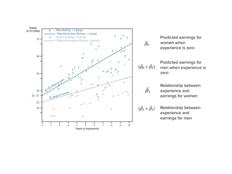
\[\hat{Wage_i}=\hat{\beta_0} + \hat{\beta_1}Experience_i + \hat{\beta_2}Male_i + \hat{\beta_3}Experience_i*Male_i\]
\(\beta_0\) - Predicted wage for women with no experience
\(\beta_0 + \beta_1\) - Relationship between experience and earnings for women
\(\beta_0 + \beta_1 + \beta_2 + \beta_3\) - Predicted Wage for men with experience
\(\beta_1\) - The effect of experience for women
\(\beta_0 + \beta_2\) - Predicted earnings for men when experience is zero
\(\beta_1 + \beta_3\) - Relationship between experience and earnings for men
8.3 Lab Questions
8.3.1 What is the effect of age on support for Trump, conditional on being a Republican? Do this with both the colon, “:”, and the “*“.
model1a <- lm(TrumpFT~Rep*Age, data=dta)
model1a
##
## Call:
## lm(formula = TrumpFT ~ Rep * Age, data = dta)
##
## Coefficients:
## (Intercept) RepTRUE Age RepTRUE:Age
## 13.1949 21.1904 0.0509 0.3780model1b <- lm(TrumpFT~Rep + Age + Rep:Age, data=dta)
model1b##
## Call:
## lm(formula = TrumpFT ~ Rep + Age + Rep:Age, data = dta)
##
## Coefficients:
## (Intercept) RepTRUE Age RepTRUE:Age
## 13.1949 21.1904 0.0509 0.37808.3.2 What is the effect of age on support for Trump, conditional on being a Democrat?
model2a <- lm(TrumpFT~Dem*Age, data=dta)
model2a
##
## Call:
## lm(formula = TrumpFT ~ Dem * Age, data = dta)
##
## Coefficients:
## (Intercept) DemTRUE Age DemTRUE:Age
## 22.5503 -9.3525 0.5281 -0.5749model2b <- lm(TrumpFT~Dem + Age + Dem:Age, data=dta)
model2b##
## Call:
## lm(formula = TrumpFT ~ Dem + Age + Dem:Age, data = dta)
##
## Coefficients:
## (Intercept) DemTRUE Age DemTRUE:Age
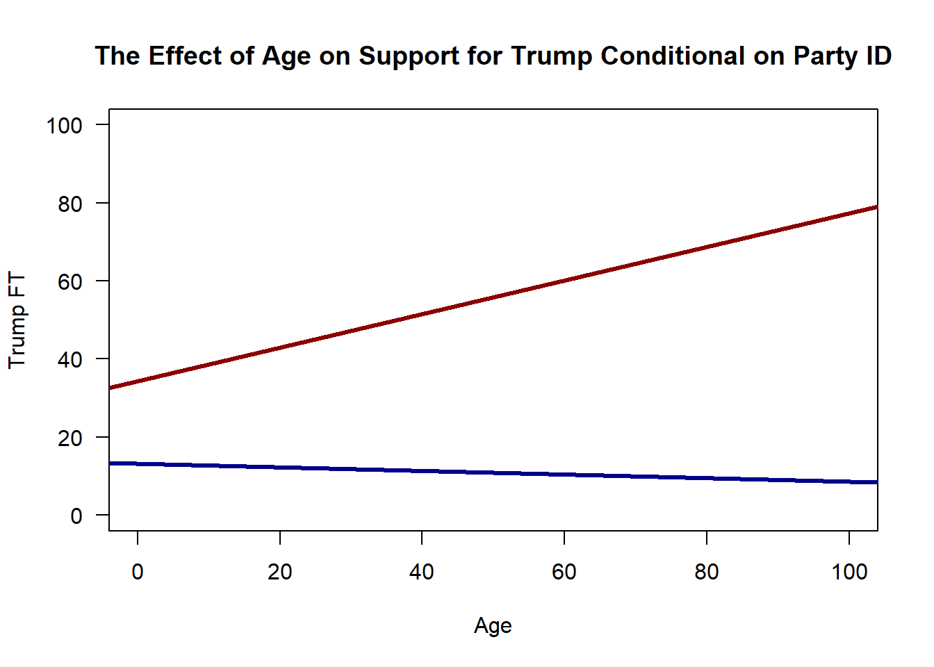
## 22.5503 -9.3525 0.5281 -0.57498.3.3 Interpret the following plot.
plot(dta$Age, dta$TrumpFT, color=dta$Rep, col=c("red", "blue"),
     main="The Effect of Age on Support for Trump Conditional on Party ID",
     xlab = "Age", ylab = "Trump FT", las=1, xlim=c(0,100), pch="")
abline(lm(TrumpFT~Age, data = subset(dta, Rep==TRUE)), col="dark red", lwd=3)
abline(lm(TrumpFT~Age, data = subset(dta, Dem==TRUE)), col="dark blue", lwd=3)
8.3.4 What are your predictions for how women may feel about Clinton, how Democrats may feel about Clinton, and how Democratic women may feel about Clinton? Then estimate the model.
Most answers will be good here. The idea is just to think about conditional effects. For example, women may approve more of Clinton because she could have been the first woman president. Democrats probably approve of Clinton because she was the Democratic nominee for president. Democratic women, then, may support Clinton EVEN more than Republican women and Democratic men. The conditional effect of being a Democrat for women will be positive.
model3 <- lm(ClintonFT~Female*Dem, data=dta)
model3
##
## Call:
## lm(formula = ClintonFT ~ Female * Dem, data = dta)
##
## Coefficients:
## (Intercept) Female DemTRUE Female:DemTRUE
## 17.690 1.114 27.621 6.8828.3.5 How do we interpret the following:
Intercept = Clinton Feelings for Male Republicans
Intercept + Beta 1 = Clinton Feelings for Female Republicans
Intercept + Beta 2 = Clinton Feelings for Male Democrats
Intercept + Beta 1 + Beta 2 + Beta 3 = Clinton Feelings for Female Democrats
Beta 1 - The Effect of Sex for Republicans
Beta 2 - The Effect of Party for Men
Beta 2 + Beta 3 - The Effect of Party for Women
Beta 1 + Beta 3 - The Effect of Sex for Democrats